Automated image analysis

Typically less than 1 − 2 % of the collected images from benthic surveys end up being annotated and processed for science purposes, and usually only a subset of pixels within each image are scored. This results in a tiny fraction of total amount of collected data being utilised, O(0.00001%). We have a number of research projects targeted at leveraging these sparse, human-annotated point labels to train Machine Learning algorithms,  in order to assist with data analysis.

A superpixel-based framework for estimating percentage cover

The following provides a brief overview of a superpixel-based framework that can be used to  efficiently extrapolate the classified results to every pixel across all the images of an entire survey. The proposed framework has the potential to broaden the spatial extent and resolution for the identification and percent cover estimation of benthic biota.

LEFT: example of annotated image scored using sparse random points. RIGHT: example of image classified using the system described here.

The following animated diagram provides an overview of the system:

Flow diagram of the proposed pipeline for sub-image classification of benthic biota. The blue arrows show the flow of unlabelled data and outputs from automated processing steps, and the red arrows show the flow of data that requires manual annotation by a human expert.

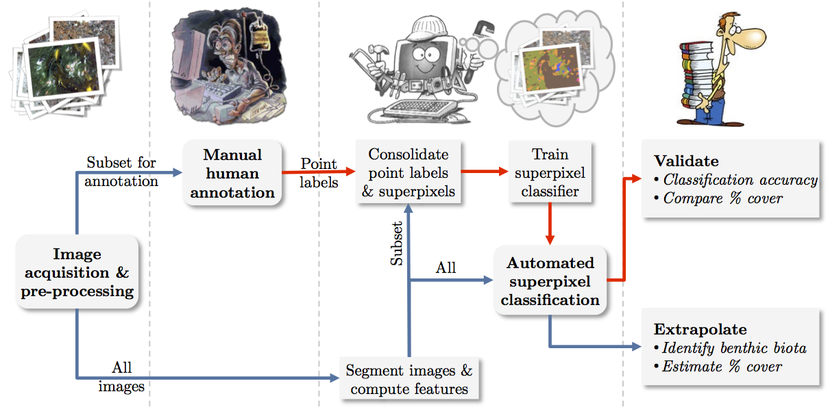
Segmentation offers some notable advantages over defining a fixed shaped and sized pixel patch for classification. For example, if a patch is positioned over a boundary between two class types, it may be difficult to determine the class label assignment, which may confound the data used for training and prediction. The figure below shows an illustrative example of this.

Classification of sub-image regions using superpixels vs square patches. (a) shows a sample image with a 100 × 100 pixel bounding box around a chosen region of interest, (b) shows a zoomed in view of the chosen region and (c) shows the class ground truth. (d) shows the classification possible with a superpixel / segmentation based approach and (e), (f) and (g) show the classification possible using non-overlapping square patches of size 100 × 100, 50 × 50 & 25 × 25 pixels, respectively

It is evident that the resolution of the classification results may also be limited by the choice of patch size and the resolution of patch positioning. Large patches may contain multiple classes making it more difficult to assign a single, specific class label and small patches may be difficult to classify as they lack context. These factors affect both the ability to classify and the resolution of the classification, which in turn may confound statistics, such as percent cover, which will be computed from the classification results. Examples of images classified using the superpixel framework are shown below.

Superpixel classification example images. The first row shows the original image examples; the second row shows labels overlaid onto segmented images (with the unlabeled superpixels coloured randomly); and the third row shows the output from the automated classifier.
Superpixel classification example images. The first row shows the original image examples; the second row shows labels overlaid onto segmented images (with the unlabelled superpixels coloured randomly); and the third row shows the output from the automated classifier.

In the image below, we can see the spatial layout of the classifier estimates vs the manually labeled points. The results show good correspondence between manual label estimates (black circles) and automated estimates (filled circles). In addition, the results appear to make sense scientifically: deeper regions are dominated by sand and the photosynthesising classes tend to be limited to the photic zone ( < 60m).

Spatial layout of percentage cover, estimated by automated superpixel classification for every pixel of all 7733 images in the survey compared to that estimated using 50 point-count of the 75 images that were scored using CPCe.

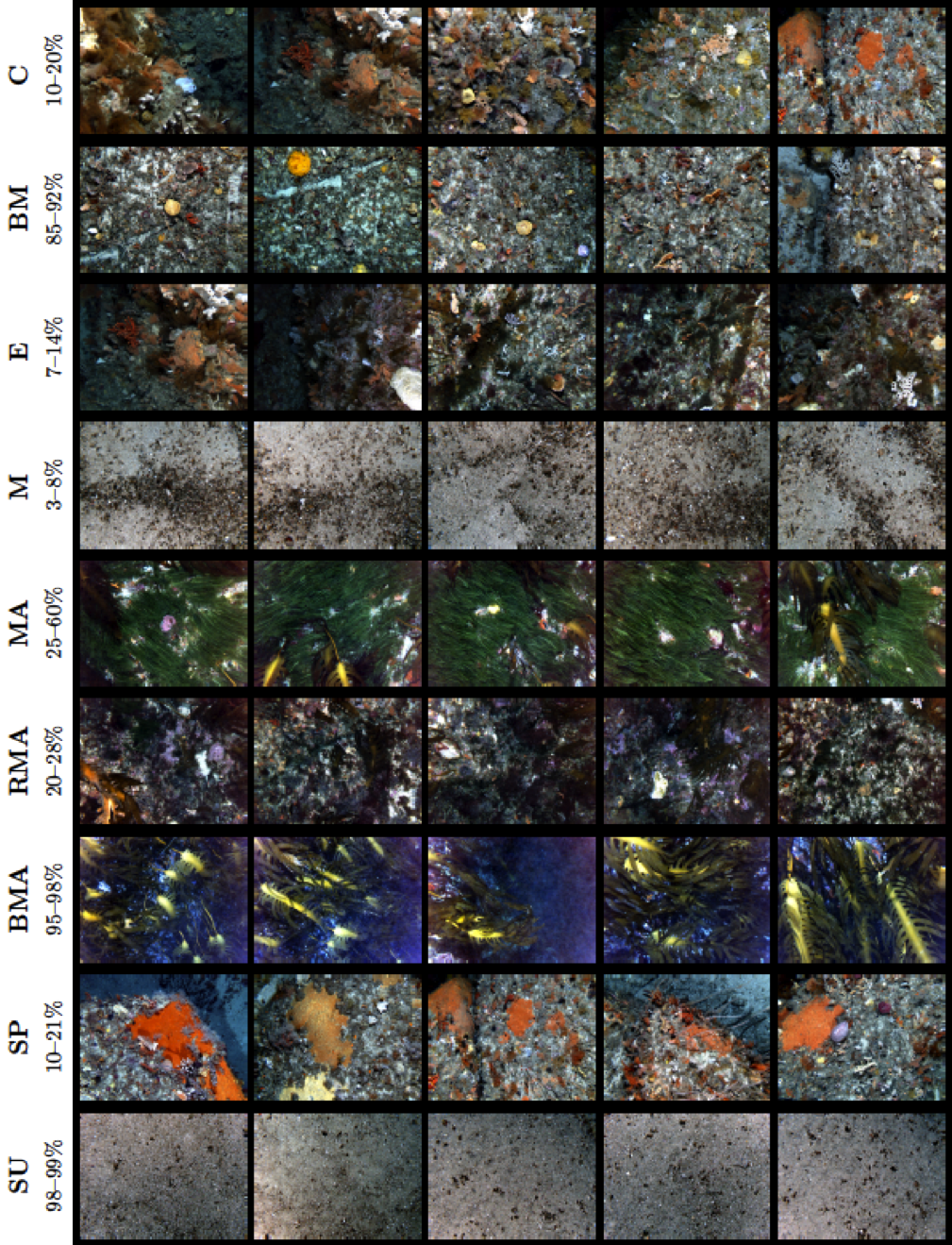
The classification results can also be used to query unannotated data. The image below show example images that have been extracted from the unlabelled data.

Non-overlapping unscored sample images for each class. Each row shows thumbnails of the 5 images that contain the highest proportion for each class. The figure also presents the range in percent cover across the images that are shown.

For more information refer to Chapter 6 of Ariell Friedman’s PhD thesis:

Friedman, A. Automated Interpretation of Benthic Stereo Imagery. Ph.D. Thesis, University of Sydney, 2013.